
Keywords: Hoeffding’s inequality; tail bounds; convex optimization
The celebrated Hoeffding’s inequality (Hoeffding, 1963Theorem 2) has been a cornerstone of probability and statistics for the last 60 years. This inequality, which we refer to as the “general Hoeffding inequality,” concerns the sum of \(n\) independent random variables, \((X_1,\ldots, X_n)\). Each variable \(X_i\) lies in some known interval \([a_i,b_i]\), for \(i\in \{1,\ldots n\}\). The general Hoeffding inequality states that the sum of these random variables, \(S=\sum_{i=1}^n X_i\), is unlikely to greatly exceed its expected value, \(\mu=\mathbb{E}[S]\). In particular, for any \(t\geq 0\), \[ \mathbb{P}(S \geq \mu+t) \leq \exp\left(-2t^2 / \sum_{i=1}^n (b_i-a_i)^2 \right).\](1) Hoeffding’s seminal work also included a less well-known bound, which is applicable only if every bounding interval is of the same length and the expected value \(\mu\) is known (Hoeffding, 1963Theorem 1). If \(a_i=0\) and \(b_i=1\) for every \(i\), then \[ \mathbb{P}(S/n \geq \mu/n+t) \leq \left(\frac{\mu/n}{\mu/n+t}\right)^{\mu+nt} \left(\frac{1-\mu/n}{1-\mu/n-t}\right)^{n-\mu-nt}.\](2) We refer to Equation (2) as the “specialized Hoeffding inequality.” Equation (2) is tighter than Equation (1) in situations where both are applicable.
In this article, we propose a computable bound on the sum of independent random variables that is applicable when the expected value of the sum is known and each random variable lies in a fixed interval with known endpoints. The lengths of these intervals may differ across variables, which prevents the direct application of the specialized Hoeffding inequality. Bounds applicable in this setting are useful for hypothesis testing regarding the sum’s expected value based on an observed realization (or, equivalently, for computing confidence intervals on the sum’s expected value).
Our key insight is that the worst-case Chernoff–Cramér bound for our setting can be easily computed to arbitrary accuracy by solving a two-dimensional convex optimization problem, yielding a tighter bound than the general Hoeffding inequality. Reliance on iterative numerical optimization prevents the use of the proposed bound in theoretical contexts that require closed-form expressions for subsequent analysis. For hypothesis testing, however, where one simply evaluates the bound numerically, a bound requiring optimization poses no impediment; standard numerical solvers find the optimum near-instantly in practice. Our approach thus complements closed-form bounds, which are looser but more amenable to theoretical manipulation. The proposed bound reduces to Equation (2) in the special case that \(a_i=0\) and \(b_i=1\) for each \(i \in \{1,\ldots,n\}\). We use simulations to demonstrate that the new bound can be much tighter than the general Hoeffding inequality when both are applicable but the specialized Hoeffding inequality is not.
The present work considers tail bounds on the sum of independent random variables when the mean of the sum is known and each variable has support in a known interval. We refer to this as a Bounded Intervals and Known Expected Sum (BIKES) assumption. There has been relatively little advance in bounds based on BIKES assumptions since the original Hoeffding bound. However, there has been substantial work on bounds from similar assumptions. We here review some of the most prominent lines of work.
First consider the assumption that \(a_i \leq X_i - \mathbb{E}[X_i] \leq b_i\) for every \(i\), with \(a_i\) and \(b_i\) known for each random variable. We refer to this as a “bounded mean deviation” (BMD) assumption.
Bounds based on a BIKES assumption can be applied whenever a BMD assumption holds to calculate the probability of a deviation from the mean: set \(Y_i = X_i - \mathbb{E}[X_i]\), observe that the BIKES assumption holds for \((Y_1,\ldots,Y_n)\), use the BIKES assumption on these variables to produce a bound for \(\mathbb{P}(\sum_{i=1}^n Y_i > t)\), then translate by \(\mu\) to obtain a bound on \(\mathbb{P}(\sum_{i=1}^n X_i > \mu+t)\). The application of the general Hoeffding inequality derived from a BMD assumption has been shown to be unnecessarily loose. For example, Hertz (2020) notes that if \(a_i\neq -b_i\) then the asymmetry can be used to produce a superior bound. On the other hand, when \(a_i=-b_i\), Bentkus (2004Corollary 1.4) provides a different bound based on a BMD assumption that is often superior to the general Hoeffding inequality.
Conversely, a bound derived from a BMD assumption can be applied whenever a BIKES assumption holds. Indeed, if a BIKES assumption gives that \(X_i\) lies in an interval of width \(b_i-a_i\), then we obtain the BMD assumption that \(X_i\) deviates from its mean by at most \(b_i-a_i\). However, in many cases \(X_i\) will in fact deviate from its mean by a quantity closer to \((b_i-a_i)/2\). Indeed, the large-deviations exponent for bounds derived from the BMD assumption alone will tend to underperform the large-deviations exponent of bounds derived from the original BIKES assumption by a factor of two.
A second line of related work considers the “constant width” (CW) assumption that each \(X_i \in [0,1]\). Bounds based on a CW assumption can be applied whenever a BIKES assumption holds by applying a single shift and rescaling all variables to lie in the unit interval. However, this yields loose bounds on the sum, as it ignores the per-variable bounds. The original specialized Hoeffding inequality is based on a CW assumption, but bounds have been improved in the meantime, for example, by Bentkus (2004Theorem 1.2). In simulations, we compare the performance of our method with Bentkus’s bounds that use a CW assumption, in which case our method reduces to Hoeffding’s specialized inequality. There has also been some work investigating how additional assumptions beyond the CW assumption can enable tighter bounds. For example, From & Swift (2013) show a refinement if \(\mu_i=\mathbb{E}[X_i]\) is known for each \(i\), and From (2023) show a refinement if \(\beta = \sum_i^n (\mu_i-\mu)^2/n\) is known.
A third line of related work focuses not on changing the assumptions of the bounded-sum problem, but on changing the proof techniques used to obtain concentration. These efforts go beyond the exponential-moment/Chernoff formulation entirely, sometimes yielding sharper tails than can be obtained from moment-generating function optimizations (Bentkus, 2002; Pinelis, 2006; cf. Talagrand, 1995). However, there are advantages to staying strictly within the exponential-moment formulation. For example, bounds based on the exponential moment apply automatically via a maximal inequality to produce bounds on the maximal value of a positive martingale. In this work, we remain within the Chernoff–Cramér exponential-moment framework, but we push it to its limit under a BIKES assumption. We identify a worst-case distribution consistent with the constraints and thereby compute the tightest Chernoff-style bound attainable in our setting.
For any scalars \(a \leq b\), let \(\mathcal{M}_{a,b}\) denote the space of probability distributions with support on \([a,b]\). For any vectors \(\boldsymbol{a}\in ({\mathbb{R}})^n\) and \(\boldsymbol{b}\in ({\mathbb{R}})^n\) and fixed value \(\mu\), let \[ \mathcal{M}_{\boldsymbol{a},\boldsymbol{b},\mu} = \left\{\boldsymbol{p} \in \prod_{i=1}^n \mathcal{M}_{a_i,b_i}:\ \sum_{i=1}^n \mathbb{E}_{X_i \sim p_i}[X_i] \leq \mu\right\}.\](3) We will say that a random vector \(\boldsymbol{X}=(X_1,\ldots X_n)\) is drawn according to a member of \((p_1,\ldots,p_n)\in \mathcal{M}_{\boldsymbol{a},\boldsymbol{b},\mu}\) if \(X_i \sim p_i\) and the variables are independent. The set \(\mathcal{M}_{\boldsymbol{a},\boldsymbol{b},\mu}\) corresponds to an assumption that the expected sum is at most \(\mu\); this milder assumption is implied by the corresponding BIKES assumption described in the previous section, but it also accommodates common hypothesis-testing settings in which the null hypothesis is that the mean at most some fixed value. It does not affect the bounds we can produce.
Our task is to produce a tail bound for the variable \(S=\sum_{i=1}^n X_i\) when \(\boldsymbol{X}\) is drawn according to \(\mathcal{M}_{\boldsymbol{a},\boldsymbol{b},\mu}\), for fixed \(\boldsymbol{a}\), \(\boldsymbol{b}\) and \(\mu\). We make two assumptions without loss of generality. First, we assume that \(b_i-a_i>0\) for each \(i\): variables with trivial support are irrelevant to bounds on \(S\). Second, we assume that each \(a_i=0\): if \(a_i\neq 0\) we transform the problem by shifting each interval left by \(a_i\) and subtracting \(\sum_{i=1}^n a_i\) from \(\mu\). Henceforth, we assume \(\boldsymbol{a}=0\) and suppress \(\boldsymbol{a}\) in our notation (e.g., we denote \(\mathcal{M}_{\boldsymbol{0},\boldsymbol{b},\mu}\) by \(\mathcal{M}_{\boldsymbol{b},\mu}\)).
Hoeffding (1963Theorem 2) provides perhaps the most famous tail bound for \(S\) when \(\boldsymbol{X}\) is drawn according to \(\mathcal{M}_{\boldsymbol{b},\mu}\). To construct this bound, Hoeffding (1963) first considers a tail bound for a particular \(\boldsymbol{p} \in \mathcal{M}_{\boldsymbol{b},\mu}\). Let \[\varphi(\boldsymbol{p},s) = \inf_{t\geq 0} \left(\sum_{i=1}^n \log \mathbb{E}_{X_i \sim p_i}[\exp(t X_i)] - ts\right).\] If \(\boldsymbol{X}\) is drawn according to any member of \(\mathcal{M}_{\boldsymbol{b},\mu}\), the Chernoff–Cramér bound gives that \(\log \mathbb{P} \left (S \geq s\right)\) is at most \(\sup_{\boldsymbol{p} \in \mathcal{M}_{\boldsymbol{b},\mu}} \varphi(\boldsymbol{p},s)\). To produce a bound that is universal for all members of \(\mathcal{M}_{\boldsymbol{b},\mu}\), Hoeffding (1963) therefore considers the quantity \[ \varphi^*_{\boldsymbol{b},\mu}(s) = \sup_{\boldsymbol{p} \in \mathcal{M}_{\boldsymbol{b},\mu}} \varphi(\boldsymbol{p},s) = \sup_{\boldsymbol{p} \in \mathcal{M}_{\boldsymbol{b},\mu}} \inf_{t\geq 0} \left(\sum_{i=1}^n \log \mathbb{E}_{X_i \sim p_i}[\exp(t X_i)] - ts\right).\](4) This leads to a tail bound for \(S\) in terms of \(\varphi^*\): \[ \mathbb{P} \left (S \geq s\right) \leq \exp(\varphi^*_{\boldsymbol{b},\mu}(s)).\](5) Equation (5) is the worst-case Chernoff–Cramér bound for a sum of independent random variables \((X_1,\ldots X_n)\) with each \(X_i \in [0,b_i]\) and \(\sum_{i=1}^n \mathbb{E}[X_i]\leq \mu\).
To compute the right-hand side of Equation (5), Hoeffding (1963) considers two different expressions for \(\varphi^*\). In one theorem, a formula for \(\varphi^*_{\boldsymbol{b},\mu}\) is provided for the special case in which \(b_1=\cdots=b_n=1\), leading to the specialized Hoeffding inequality, Equation (2). In another theorem, an upper bound is produced for \(\varphi^*_{\boldsymbol{b},\mu}\) in the general case of arbitrary \(\boldsymbol{b}\), namely, \(\varphi^*_{\boldsymbol{b},\mu}(s)\leq -2(s-\mu)^2/\sum_{i=1}^n b_i^2,\) leading to the general Hoeffding inequality.
Our contribution in the next section is to show how \(\varphi^*\) can be exactly computed for arbitrary interval lengths \(\boldsymbol{b}\). By substituting this exact value of \(\varphi^*\) into Equation (5), an improved tail bound for the sum of bounded independent random variables follows.
We now show that \(\varphi^*\) (cf. Equation (4)) can be computed by solving a two-dimensional convex optimization problem. We begin by expressing \(\varphi^*\) as the solution to a high-dimensional convex optimization problem and then demonstrate how to reduce this problem to a more tractable two-dimensional problem.
Equation (4) defines \(\varphi^*\) as the solution to a maximin problem that involves maximizing over distributions and minimizing over values of \(t>0\). The inner one-dimensional minimization over \(t\) can be commuted with the outer infinite-dimensional maximization over \(\boldsymbol{p}\in\mathcal{M}_{\boldsymbol{b},\mu}\). Once the minimization and maximization operators have been commuted, the inner problem reduces to a finite-dimensional optimization problem. This leads to a new expression for \(\varphi^*\), as shown below.
Theorem 1. Fix \(\boldsymbol{b}=(b_1,\ldots b_n)\), \(\mu \in [0,\sum_{i=1}^n b_i]\), and \(s \in [0,\sum_{i=1}^n b_i]\). Let \[\begin{aligned} T_{(=)}& =\left\{\tau\in \prod_{i=1}^n [0,b_i] : \sum_{i=1}^n \tau_i = \mu\right\} & T_{(\leq)}& =\left\{\tau\in \prod_{i=1}^n [0,b_i] : \sum_{i=1}^n \tau_i \leq \mu\right\}.\end{aligned}\] Then, taking \(T=T_{(=)}\) or \(T=T_{(\leq)}\), \(\varphi^*_{\boldsymbol{b},\mu}(s)\) from Equation (4) can be expressed as \[\begin{aligned} \varphi^*_{\boldsymbol{b},\mu}(s) &= \inf_{t\geq 0} \left(\max_{\tau \in T} \sum_{i=1}^n \log\left(1+\tau_i (\exp(b_i t)-1)/b_i \right) - ts\right).\end{aligned}\]
The high-dimensional minimax problem from Theorem 1 can be reduced to a two-dimensional convex optimization problem.
Theorem 2. Fix \(\boldsymbol{b}=(b_1,\ldots b_n)\), \(\mu \in [0,\sum_{i=1}^n b_i]\), and \(s \in [0,\sum_{i=1}^n b_i]\). Let \(\xi(b,t) = (\exp(bt)-1)/b\), \[\tau^*_i(t,\lambda) = \min\left(\max\left(\frac{\xi(b_i,t)-\lambda}{\xi(b_i,t)\lambda},0\right),b_i\right),\] and \[g(t,\lambda;s) = \sum_i \log\left(1+\xi(b_i,t)\tau_i^*(t,\lambda)\right) + \lambda\left(\mu - \sum_i \tau_i^*(t,\lambda)\right)- ts.\] Then, \(g\) is convex and \(\varphi^*_{\boldsymbol{b},\mu}(s)\) from Equation (4) can be expressed as \[\varphi^*_{\boldsymbol{b},\mu}(s) = \inf_{t,\lambda \geq 0} g(t,\lambda;s).\] Moreover, the mapping \(t \mapsto \min_\lambda g(t,\lambda;s)\) is convex, and the mapping \(\lambda \mapsto g(t,\lambda;s)\) is convex for each \(t \geq 0\).
This theorem suggests two methods for computing \(\varphi^*\). One method involves directly minimizing the two-dimensional convex function \(t,\lambda \mapsto g(t,\lambda;s)\) and the other involves minimizing the one-dimensional convex function \(t \mapsto \min_\lambda g(t,\lambda;s)\). Because each evaluation of the objective function of the latter requires solving a different one-dimensional convex optimization problem, we use the first method in our simulations.


We use simulations to assess the degree of improvement over the general Hoeffding inequality. First, we sample a vector of interval lengths, \(\boldsymbol{b} \in \mathbb{R}^{100}\), uniformly at random from the set of lengths such that \(B=\sum_{i=1}^{100} b_i=1\). We define \(S\) to be the sum of 100 independent random variables, \((X_1,\ldots,X_{100})\), where each \(X_i\) is constrained to the interval \([0,b_i]\) for \(i\in \{1,\ldots,100\}\). The value of \(n\) could affect the tightness of all bounds, but in the supplementary material we show the effect is negligible for this kind of simulation. The overall scaling of the \(b_i\) values does not affect tightness: what is relevant is the relative sizes of the intervals, so we normalize the intervals so that their maximum possible sum is 1.
For any fixed value of \(\mu\) and any value \(s \geq \mu\), our new results provide an upper bound on \(\mathbb{P}(S>s)\), assuming \(\mathbb{E}[S]\leq \mu\). The general Hoeffding inequality can also be used to produce a bound on \(\mathbb{P}(S>s)\), offering a natural point of comparison. We also compare with the two Bentkus bounds (Bentkus, 2004): Theorem 1.2 is applicable in the CW setting and requires all bounding intervals to be of the same size, while Corollary 1.4 is applicable in the BMD setting and provides per-variable scaling but requires centering information. To apply Theorem 1.2 to heterogeneous intervals, we rescale all variables so that they lie within \([0, \max_i b_i]\). For Corollary 1.4, we apply it using only the overall centering \(S - \mu\). These bounds on \(\mathbb{P}(S>s)\) have practical implications, such as facilitating hypothesis testing for \(\mathbb{E}[S]\leq \mu\) given an observed realization of \(S\).
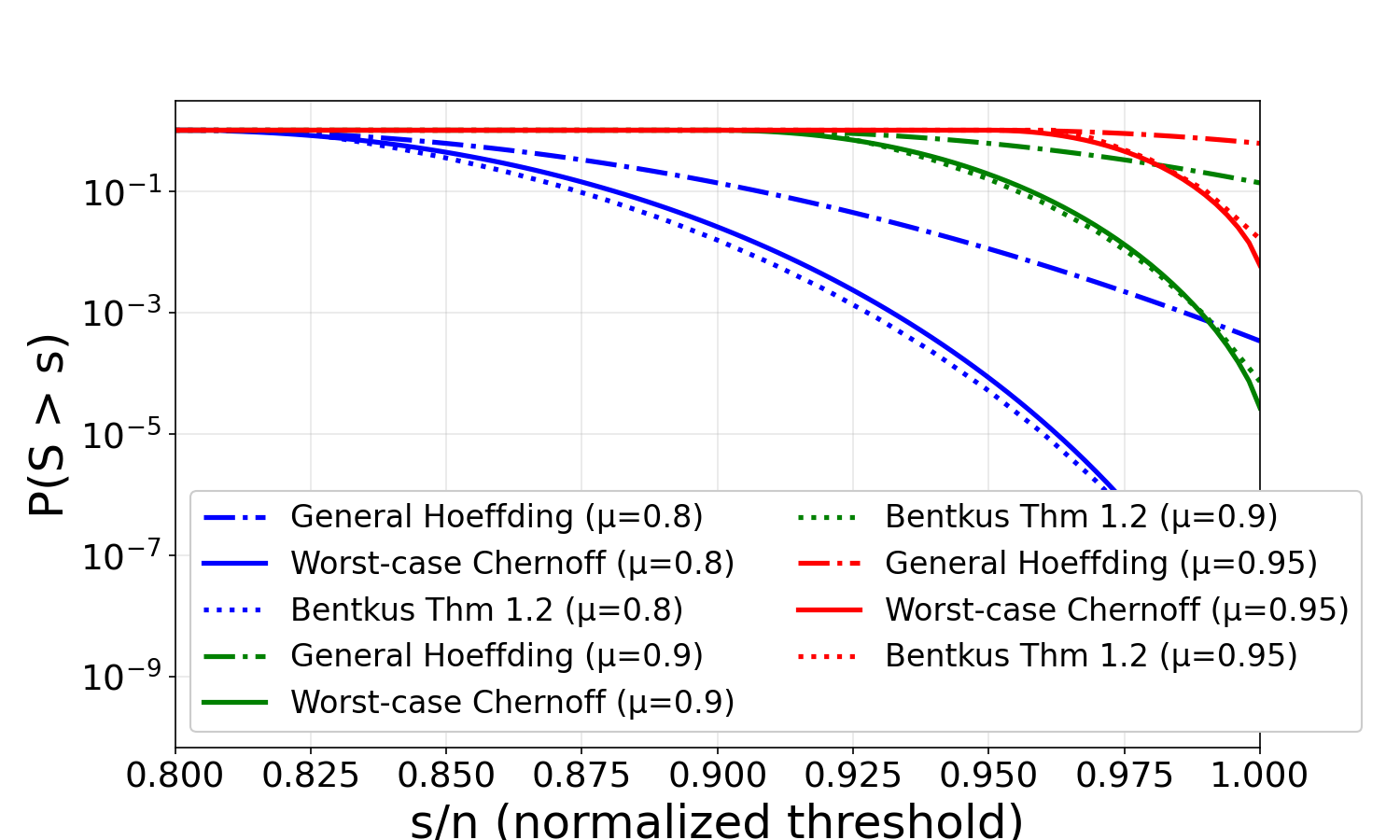
Figure 2 compares our new worst-case Chernoff bounds with the general Hoeffding inequality and both Bentkus bounds for \(\mu \in \{0.8, 0.9, 0.95\}\), showing how they vary as a function of \(s\). In many cases, our bounds are orders of magnitude tighter than those derived from the general Hoeffding inequality, demonstrating their advantage in tail estimation. Neither Bentkus bound performs as well as our method in the heterogeneous case: Theorem 1.2 effectively treats all intervals as having the maximum width (a consequence of applying a CW bound), while Corollary 1.4 has a larger multiplicative constant and, as a BMD-type bound, does not fully exploit the heterogeneity.
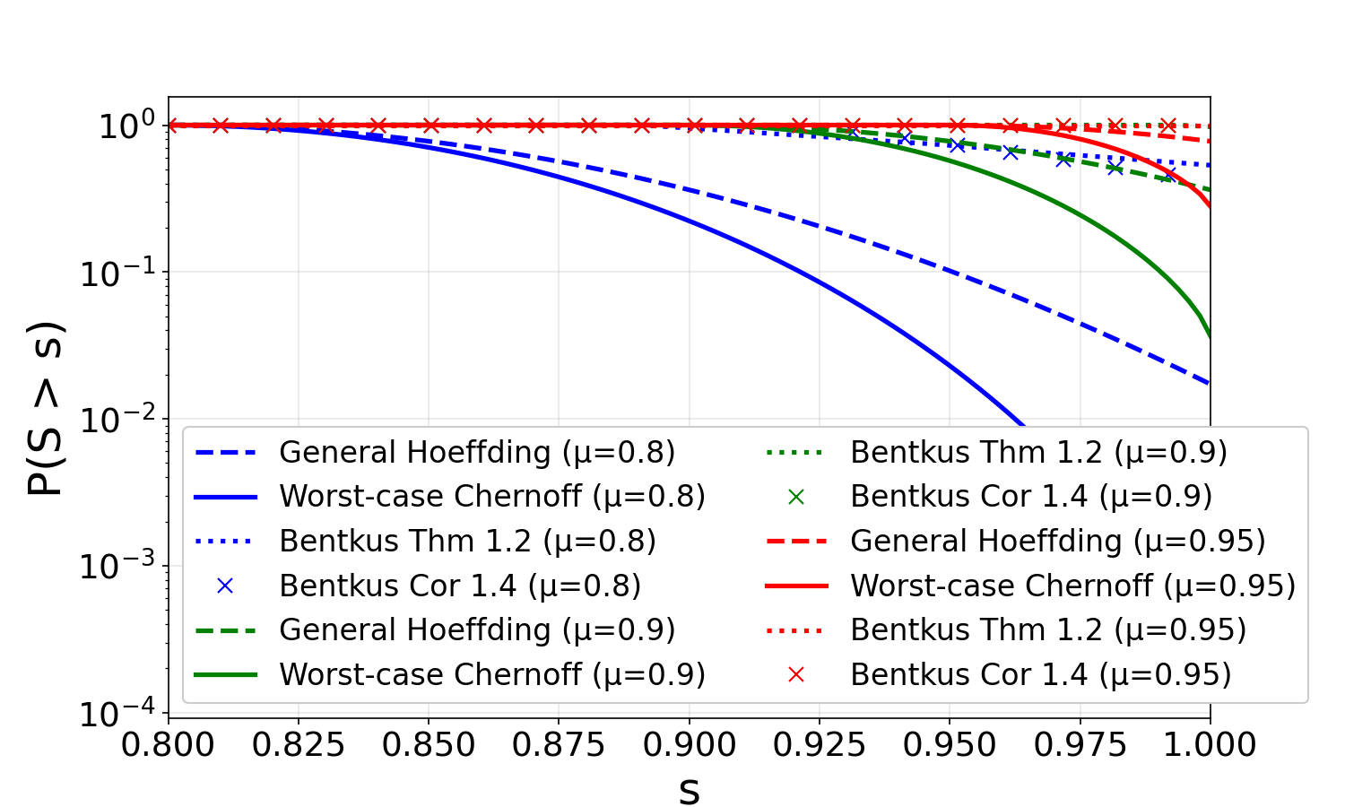
To verify that our bounds perform well even when the Bentkus bounds are directly applicable, we also consider the case of homogeneous intervals where all \(b_i = 1\), which corresponds to the CW setting. Figure 2 shows this comparison. In this setting, our new worst-case Chernoff bounds coincide with the specialized Hoeffding inequality (Equation (2)), as guaranteed by Theorem 2. Both our bounds and Bentkus Theorem 1.2 are much tighter than the general Hoeffding inequality, demonstrating that all refined methods provide substantial improvements when applicable. The key advantage of our worst-case Chernoff approach is that it extends naturally to heterogeneous intervals without requiring any rescaling or centering information beyond the overall mean.
SUPPLEMENTARY MATERIAL
Code for solving the two-dimensional convex optimization problem involved in the new bound, together with demonstrations of its use. (Jupyter notebook)
plots similar to those in Figure 1, with difference choices for \(n\) (Document)
To prove Theorem 1, it is convenient to view \(\mathcal{M}_{\boldsymbol{b},\mu}\) from Equation (3) as a subset of a topological vector space. For any scalar \(b\geq 0\), let \(\mathcal{M}_b\) denote the space of probability measures with support on \([0,b]\). Endowing \(\mathcal{M}_b\) with the weak-\(*\) topology, we may view \(\mathcal{M}_b\) as a subset of a topological vector space of measures. Note that \(\mathcal{M}_b\) is compact and convex. For any values \(\boldsymbol{b}\in ({\mathbb{R}^+})^n\) and fixed expected value \(\mu\), let \[\mathcal{M}_{\boldsymbol{b},\mu} = \left\{\boldsymbol{p} \in \prod_i \mathcal{M}_{b_i}:\ \sum_i\mathbb{E}_{X_i \sim p_i}[X_i] \leq \mu\right\}.\] We emphasize that an object \(\boldsymbol{p} \in \prod_{i=1}^n \mathcal{M}_{b_i}\) is not itself a distribution on \(n\) independent random variables: it is merely a collection of \(n\) marginal distributions. If \(\boldsymbol{p} \in \mathcal{M}_{\boldsymbol{b},\mu}\) then \(\boldsymbol{p}=(p_1,\ldots, p_n)\) where each \(p_i \in \mathcal{M}_{b_i}\). Any convex combination of a pair of such objects \((\boldsymbol{p},\boldsymbol{q}) \in \mathcal{M}_{\boldsymbol{b},\mu}\) would then be computed as \((\alpha \boldsymbol{p}+(1-\alpha)\boldsymbol{q})=(\alpha p_1+(1-\alpha) q_1,\ldots, \alpha p_n+(1-\alpha) q_n)\). This seemingly excessive formality is necessary to clarify that \(\mathcal{M}_{\boldsymbol{b},\mu}\) is, in fact, convex. This convexity is essential for proving the results that follow. Note that for ease of exposition, we may sometimes say that a random vector \(\boldsymbol{X}\) is drawn according to \(\boldsymbol{p}\), by which we mean that the collection of random variables \(\{X_1,\ldots X_n\}\) is mutually independent and each \(X_i \sim p_i\).
Theorem 1 (Restatement of Theorem 3.1). Fix \(\boldsymbol{b}=(b_1,\ldots b_n)\), \(\mu \in [0,\sum_{i=1}^n b_i]\), and \(s \in [0,\sum_{i=1}^n b_i]\). Let \[\begin{aligned} T_{(=)}& =\left\{\tau\in \prod_{i=1}^n [0,b_i] : \sum_{i=1}^n \tau_i = \mu\right\} & T_{(\leq)}& =\left\{\tau\in \prod_{i=1}^n [0,b_i] : \sum_{i=1}^n \tau_i \leq \mu\right\}.\end{aligned}\] Then, taking \(T=T_{(=)}\) or \(T=T_{(\leq)}\), \(\varphi^*_{\boldsymbol{b},\mu}(s)\) from Equation (4) can be expressed as \[\begin{aligned} \varphi^*_{\boldsymbol{b},\mu}(s) &= \inf_{t\geq 0} \left(\max_{\tau \in T} \sum_{i=1}^n \log\left(1+\tau_i (\exp(b_i t)-1)/b_i \right) - ts\right).\end{aligned}\]
Proof. Fix \(s\). Let \(\xi(b,t)=(\exp(bt)-1)/b\). Let \[f(t,\boldsymbol{p})=\sum_{i=1}^n\log \mathbb{E}_{X_{i}\sim p_{i}}[\exp(tX_{i})]-ts.\] Our object of interest is \(\inf_{t}\max_{\boldsymbol{p}}f(t,\boldsymbol{p})\). Our first step is to reverse the order of the minimization and maximization by applying Sion’s minimax theorem (Komiya, 1988). We observe the following: \(f\) is convex with respect to \(t\) (as it is the sum of cumulant generating functions), \(f\) is concave with respect to \(\boldsymbol{p}\) (due to Jensen’s inequality), \(f\) is continuous with respect both \(\boldsymbol{p}\) and \(t\), \(\mathcal{M}_{\boldsymbol{b},\mu}\) is both convex and compact, and \([0,\infty)\) is convex (though not compact). Sion’s minimax theorem thus shows that \[\inf_{t\geq0}\sup_{\boldsymbol{p}\in\mathcal{M}_{\boldsymbol{b},\mu}}f(t,\boldsymbol{p})=\sup_{\boldsymbol{p}\in\mathcal{M}_{\boldsymbol{b},\mu}}\inf_{t\geq0}f(t,\boldsymbol{p}).\] For any fixed \(t\), the maximization of \(f\) may be reduced to a finite-dimensional problem. First, we rewrite the maximization problem by introducing auxiliary variables, as follows: \[\begin{gathered} \max_{\boldsymbol{p},\tau} f(t,\boldsymbol{p}) \qquad \mathrm{s.t.}\qquad \tau_{i}\in[0,b_i],\ p_{i}\in\mathcal{M}_{b_i},\ \tau_{i}=\mathbb{E}_{X_{i}\sim p_{i}}\left[X_{i}\right],\ \sum_{i=1}^n\tau_{i} \leq \mu\end{gathered}\] For any fixed \(\tau\), Hoeffding (Hoeffding, 1963proof of Theorem 1) showed that the cumulant generating functions can be maximized by setting each \(p_{i}\) to be a scaled Bernoulli random variable, namely \[p_{i}=\delta_{0}\left(1-\frac{\tau_{i}}{b_i}\right)+\delta_{b_i}\frac{\tau_{i}}{b_i}\] where \(\delta_{x}\) represents the point mass at \(x\). Under this distribution, \[\log \mathbb{E}_{X_i \sim p_{i}}\left[\exp\left(tX_{i}\right)\right]=\log\left(1+\xi(b_i,t)\tau_{i}\right).\] Summing over \(i\), we obtain that \[\begin{gathered} \varphi^*_{\boldsymbol{b},\mu}(s) = \inf_{t\geq 0} \left(\max_{\tau\in \prod_{i=1}^n [0,b_i]: \sum_{i=1}^n \tau_i \leq \mu} \sum_{i=1}^n \log\left(1+\tau_i (\exp(b_i t)-1)/b_i \right) - ts\right).\end{gathered}\] This proves the statement in the theorem regarding \(T_{(\leq)}\). To show the corresponding statement for \(T_{(=)}\), note that the objective is coordinate-wise non-decreasing in \(\tau\) (strictly increasing if \(t>0\)). Hence, if a maximizer \(\tau^\star\) under \(\sum_i\tau_i\le \mu\) had slack, i.e. \(\sum_i\tau_i^\star<\mu\), then since \(\mu\le\sum_i b_i\) there exists some \(j\) with \(\tau_j^\star<b_j\); increasing \(\tau_j^\star\) by \(\varepsilon=\min\{b_j-\tau_j^\star,\ \mu-\sum_i\tau_i^\star\}>0\) preserves feasibility and (in case \(t>0\)) strictly increases the objective, a contradiction. Thus, the maximum is attained at \(\sum_i\tau_i=\mu\) (and when \(t=0\) the objective is constant, so the value is unchanged regardless of \(\tau\)). ◻
Theorem 2 (Restatement of Theorem 3.2). Fix \(\boldsymbol{b}=(b_1,\ldots b_n)\), \(\mu \in [0,\sum_{i=1}^n b_i]\), and \(s \in [0,\sum_{i=1}^n b_i]\). Let \(\xi(b,t) = (\exp(bt)-1)/b\), \[\tau^*_i(t,\lambda) = \min\left(\max\left(\frac{\xi(b_i,t)-\lambda}{\xi(b_i,t)\lambda},0\right),b_i\right),\] and \[g(t,\lambda;s) = \sum_i \log\left(1+\xi(b_i,t)\tau_i^*(t,\lambda)\right) + \lambda\left(\mu - \sum_i \tau_i^*(t,\lambda)\right)- ts.\] Then, \(g\) is convex and \(\varphi^*_{\boldsymbol{b},\mu}(s)\) from Equation (4) can be expressed as \[\varphi^*_{\boldsymbol{b},\mu}(s) = \inf_{t,\lambda \geq 0} g(t,\lambda;s).\] Moreover, the mapping \(t \mapsto \min_\lambda g(t,\lambda;s)\) is convex, and the mapping \(\lambda \mapsto g(t,\lambda;s)\) is convex for each \(t \geq 0\).
Proof. Let \(T=\{\tau\in \prod_{i=1}^n [0,b_i]: \sum_{i=1}^n \tau_i = \mu\}\). Recall from Theorem 1 that \[\begin{gathered} \varphi^*_{\boldsymbol{b},\mu}(s) = \inf_{t\geq 0} \left(\max_{\tau \in T} \sum_{i=1}^n \log\left(1+\tau_i (\exp(b_i t)-1)/b_i \right) - ts\right).\end{gathered}\] For any fixed \(t\geq0\), we begin by rewriting the inner maximization problem in terms of \[f(\tau;t)=\begin{cases} \sum_{i=1}^n\log\left(1+\xi(b_i,t)\tau_{i}\right)-ts & \mathrm{if}\ \tau\in\prod_{i}[0,b_i]\\ -\infty & \mathrm{else}. \end{cases}\] The inner maximization problem is thus equivalent to \[\max_{\tau:\ \sum_{i=1}^n\tau_{i}=\mu}f(\tau;t).\] The associated Lagrangian function is given by \[\mathcal{L}(\tau,\lambda;t)=\sum_{i=1}^n\log\left(1+\xi(b_i,t)\tau_{i}\right)+\lambda\left(\mu-\sum_{i=1}^n\tau_{i}\right)-ts.\] For any fixed \(t\geq0\), observe that \(\xi(b_i,t)\) is positive and thus \(\tau\mapsto\mathcal{L}\left(\tau,\lambda;t\right)\) is concave. The argument maximizing \(\tau\mapsto\mathcal{L}(\tau,\lambda;t)\) is given by \(\tau_{i}^{*}(t,\lambda)\). Thus \(g(t,\lambda;s)=\max_{\tau}\mathcal{L}(\tau,\lambda;t)\), the Lagrangian dual for a convex optimization problem with convex constraints. There is at least one feasible point, namely \(\tau_{i}=b_i\mu/\sum_{j}b_{j}\), so strong duality holds and \[\max_{\substack{\tau\in\prod_{i}[0,b_i]\\ \sum_{i=1}^n\tau_{i}=\mu } }\sum_{i=1}^n\log\left(1+\xi(b_i,t)\tau_{i}\right)-ts=\inf_{\lambda}g(t,\lambda;s)\] as desired.
We now demonstrate that \(g\) is convex. First, observe that \(\mathcal{L}\) is affine in \(\lambda\) and convex in \(t\). Thus \(g\) is a pointwise maximum of a family of convex functions: it is convex.
Finally, we demonstrate that \(t\mapsto\inf_{\lambda}g(t,\lambda;s)\) is convex. Observe that, for any fixed \(\tau_{i}\geq0\), the mapping \[t\mapsto\sum_{i=1}^n\log\left(1+\xi(b_i,t)\tau_{i}\right)-ts\] is convex in \(t\). Thus \(\inf_{\lambda}g(t,\lambda;s)\) is also the pointwise maximum of a family of convex functions: it is also convex. ◻